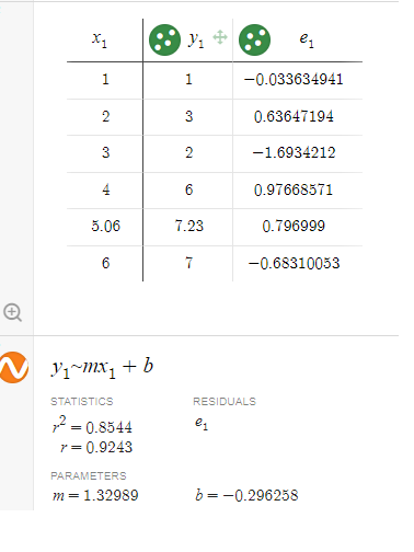
Linear regression is a good visualization to explain machine learning. The machine or computer actually did not learn by itself to discover the generalized line equation in slope form. In this example you gave the computer six (6) training data points to approximate the best line equation.

Using only two dimensions machine or computer can predict or inference the correct answer. Dimension 1 is represented by letter variable x in x-axis. Variable x is also called predictor input or independent variable.

Dimension 2 is represented by letter variable y in y-axis. Variable y is also called the predicted output or dependent variable.

credit to : Desmos Graphing by Sam Ortega 5/28/2022

Then you select the best fit linear equation algorithm that best describe the relationship between the two given dimensions x and y variables. The discovered relationship is summarize by the line slope equation y = 1.329x - 0.296. This equation is now called the machine learning model at that time using six (6) training data point. This linear equation is used to predict the output value of y given the input value of x.

But other task like image identification, classification, object detection, information retrieval, search, fraud detection, anomaly detection, voice to text, and text to voice translation have more than two dimensions or parameters which linear regression algorithm is not good at. So, machine learning engineer, AI research scientist, data scientist created new algorithm to automate the iteration of undefined and hidden pattern. Because it is still hard to discover the generalized pattern or equation, hence, the algorithm is referred to as black box. Since the dimensions could be in thousands, millions, billions or even trillion of parameters we need the machine to help us discover the pattern.

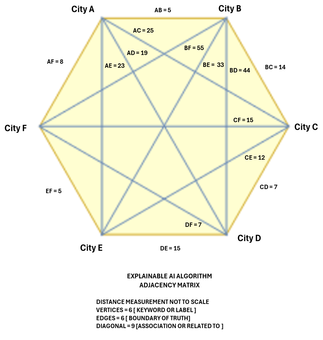
Emerging Algorithm to Watch: Adjacency Matrix Algorithm

The Adjacency Matrix Algorithm is revolutionizing various fields:

Graph Representation: Efficiently represents graphs for better visualization and analysis.

Connectivity Analysis: Enhances understanding of network connections.

Graph Algorithms: Powers algorithms like Dijkstra’s, Floyd-Warshall, and Kruskal’s for optimal solutions.

Image Processing: Improves image recognition by analyzing pixel relationships.

Social Network Analysis: Unveils insights into social connections and interactions.

Network Routing: Optimizes data routing in networks.

Urban Traffic Planning: Aids in designing smarter traffic systems.



Example of Graph Adjacency Matrix Algorithm



Graph Neural Network (GNN)
Graph Convolutional Newtork (GCN)
Graph Attention Network (GAT)
DeepWalk
Node2Vec
PageRank
Label Propagation Algorithm (LPA)

Again the basic principle is the same, the machine or computer did not learn by itself, humans give the training inputs to discover the pattern or relationship. The hidden pattern discovered by machine appears to be very hard to trace for auditing so human can see where the errors happen. The machine learning is now behaving like a human brain where you can not see the many series of mathematical equations it selected to deliver the correct output.

But expertise of human brain is achieved by continuous training until it can repeat the correct output. Then when the output is proven to be wrong the human brain will document the known input that resulted to a wrong output and document the event as known exception where the answer or output is not valid or wrong. Then human brain will do another training to discover the root cause why the answer or output is wrong.

Similarly machine learning hidden or black box model will need another training when its predicted output or answer is no longer valid due to new added informations that were not available at the time of training.

Scatterplot is a good visualization of the coefficient of relationship between the input data (x) and the output or predicted value(y).

Scatterplot is the first evidence you need to show that there is a linear relationship that exist between the input data (x) and the output or predicted value(y). If you can't show it. Then your assumption of linear relationship is questionable and can't be used for predicting the output.

In Excel the r-value or the relationship coefficient between the input x and output tells you the confidence level that a linear relationship exist. If r value = 0.9998 it means there is a very high confidence that a direct linear relationship exist. Therefore you can use the x input data to predict the value of output y.

If r value = 0.3451 it means there is a low confidence that a direct linear relationship exist and therefore the x value input can't be used for predicting the output value of y.

credit to : Desmos Graphing by Sam Ortega 5/28/2022

Different Type of Machine
Learning Algorithm

Understanding Latent Space in
Machine Learning

Many Types of Regression

How to tell if a person has supporting evidence as machine learning subject matter expert